import numpy as np
import pandas as pd
import matplotlib.pyplot as plt
import seaborn as sns
import statsmodels.api as sm
plt.rcParams['font.family'] = 'Noto Sans CJK JP'  # または利用可能な日本語フォント名

df = sm.datasets.get_rdataset("wage1", "wooldridge").data回帰分析
回帰分析の例として,教育の収益率の推定をやってみよう。
パッケージとデータの読込み
ここで用いるのは,Wooldridgeのテキストで使われている”wage1”というデータ。statsmodelsで読み込むことができる。元データは,1976年のアメリカのCurrent Population Survey。古いデータではあるが,練習用には便利。
データの概要
データの概要は,info()メソッドで確認できる。
df
df.info()
<class 'pandas.core.frame.DataFrame'>
RangeIndex: 526 entries, 0 to 525
Data columns (total 24 columns):
# Column Non-Null Count Dtype
--- ------ -------------- -----
0 wage 526 non-null float64
1 educ 526 non-null int64
2 exper 526 non-null int64
3 tenure 526 non-null int64
4 nonwhite 526 non-null int64
5 female 526 non-null int64
6 married 526 non-null int64
7 numdep 526 non-null int64
8 smsa 526 non-null int64
9 northcen 526 non-null int64
10 south 526 non-null int64
11 west 526 non-null int64
12 construc 526 non-null int64
13 ndurman 526 non-null int64
14 trcommpu 526 non-null int64
15 trade 526 non-null int64
16 services 526 non-null int64
17 profserv 526 non-null int64
18 profocc 526 non-null int64
19 clerocc 526 non-null int64
20 servocc 526 non-null int64
21 lwage 526 non-null float64
22 expersq 526 non-null int64
23 tenursq 526 non-null int64
dtypes: float64(2), int64(22)
memory usage: 98.8 KB526人の労働者について24の変数が格納されている。変数の中には,基本的な変数の対数変換や,二乗なども含まれている (通常これらは自分で作成する)。
ここでは,賃金と修学年数との関係に注目する。賃金と修学年数の分布 (ヒストグラム)と散布図を描いてみよう。
sns.histplot(
    df['educ'],
    discrete=True,  # 離散変数として扱う
    edgecolor="black"
)
plt.xlabel('修学年数')
plt.locator_params(axis='x', integer=True)  # X軸の目盛りを整数に
plt.show()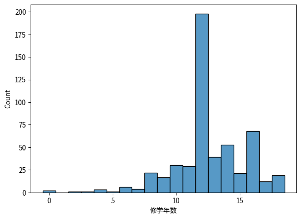
sns.histplot(
    df['wage'],
    edgecolor="black"
)
plt.xlabel('時間あたり賃金 (ドル)')
plt.show()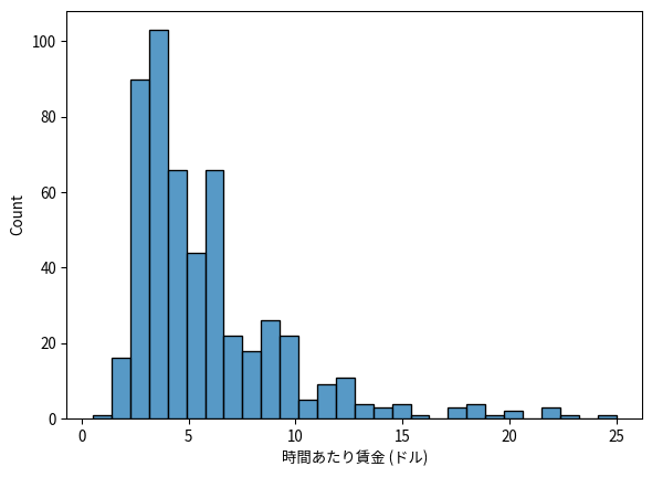
sns.scatterplot(
    x='educ',
    y='wage',
    alpha=0.5,
    data=df
)
plt.xlabel('修学年数')
plt.ylabel('時間あたり賃金 (ドル)')
plt.show()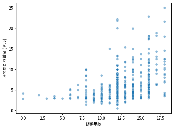
回帰分析
散布図を見ると,教育水準が高いほど時間あたり賃金も高いことがわかる。ここで,われわれが知りたいのは,修学年数が1年増加すると,どの程度賃金が上昇するかということである。
そのため,散布図で示された修学年数と時間あたり賃金との関係に,最も良く当てはまる直線 (回帰直線)を引いてみよう。
sns.regplot(data=df, x='educ', y='wage', line_kws={'color': 'red', 'linestyle': '--'})
plt.xticks(np.arange(0, df['educ'].max()+1, 1))
plt.show()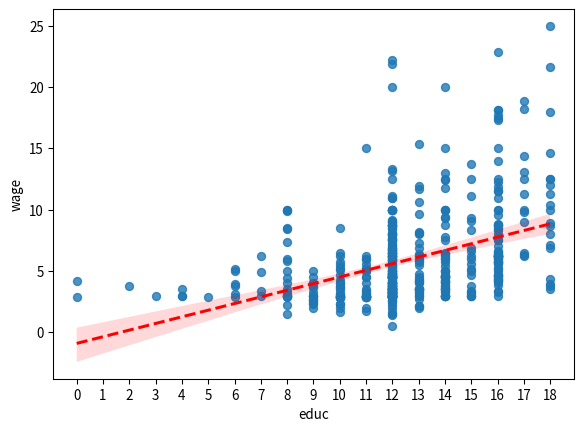
回帰直線は右上がりであり,修学年数が増加すると時間あたり賃金が上昇するという関係を表している。回帰直線の式は,最小二乗法 (OLS)で求める。
X = df['educ']
y = df['wage']
X = sm.add_constant(X)  # 定数項を追加

model = sm.OLS(y, X).fit()
print(model.summary())
OLS Regression Results
==============================================================================
Dep. Variable: wage R-squared: 0.165
Model: OLS Adj. R-squared: 0.163
Method: Least Squares F-statistic: 103.4
Date: Thu, 15 Jan 2026 Prob (F-statistic): 2.78e-22
Time: 00:15:05 Log-Likelihood: -1385.7
No. Observations: 526 AIC: 2775.
Df Residuals: 524 BIC: 2784.
Df Model: 1
Covariance Type: nonrobust
==============================================================================
coef std err t P>|t| [0.025 0.975]
------------------------------------------------------------------------------
const -0.9049 0.685 -1.321 0.187 -2.250 0.441
educ 0.5414 0.053 10.167 0.000 0.437 0.646
==============================================================================
Omnibus: 212.554 Durbin-Watson: 1.824
Prob(Omnibus): 0.000 Jarque-Bera (JB): 807.843
Skew: 1.861 Prob(JB): 3.79e-176
Kurtosis: 7.797 Cond. No. 60.2
==============================================================================
Notes:
[1] Standard Errors assume that the covariance matrix of the errors is correctly specified.すなわち,回帰直線の式は以下で表される。 \[ \widehat{wage} = -0.905 + 0.541 educ \] したがって,修学年数が1年増加すると,時間あたり賃金は0.54ドル増加することがわかる。
対数変換
次に,時間あたり賃金の対数値を被説明変数として回帰分析を行ってみよう。
X = df[['educ']]
y = df['lwage']
X = sm.add_constant(X)  # 定数項を追加

model_multi = sm.OLS(y, X).fit()
print(model_multi.summary())
OLS Regression Results
==============================================================================
Dep. Variable: lwage R-squared: 0.186
Model: OLS Adj. R-squared: 0.184
Method: Least Squares F-statistic: 119.6
Date: Thu, 15 Jan 2026 Prob (F-statistic): 3.27e-25
Time: 00:15:05 Log-Likelihood: -359.38
No. Observations: 526 AIC: 722.8
Df Residuals: 524 BIC: 731.3
Df Model: 1
Covariance Type: nonrobust
==============================================================================
coef std err t P>|t| [0.025 0.975]
------------------------------------------------------------------------------
const 0.5838 0.097 5.998 0.000 0.393 0.775
educ 0.0827 0.008 10.935 0.000 0.068 0.098
==============================================================================
Omnibus: 11.804 Durbin-Watson: 1.801
Prob(Omnibus): 0.003 Jarque-Bera (JB): 13.811
Skew: 0.268 Prob(JB): 0.00100
Kurtosis: 3.586 Cond. No. 60.2
==============================================================================
Notes:
[1] Standard Errors assume that the covariance matrix of the errors is correctly specified.すなわち,回帰直線の式は, \[ \widehat{\log (wage)} = 0.584 + 0.083 educ \] 修学年数が1年増加すれば,時間あたり賃金の対数値が0.08増加する。これは,修学年数が1年増加すれば賃金が約8%増加するとことを意味する。このように,被説明変数として賃金の対数値を用いることで,修学年数の係数を1年あたりの教育の収益率と見なすことができる。
従属変数と独立変数にレベル (もとの値)を使うか,log (対数)を使うかによって,回帰係数の解釈は以下のようになる。
| 従属変数 | 独立変数 | 係数\(\beta\)の解釈 |
|---|---|---|
| \(y\) | \(x\) | 限界効果 (\(x\)が1単位変化 → \(y\)は\(\beta\)単位変化) |
| \(\log y\) | \(x\) | \(x\)が1単位変化 → \(y\)は\(\beta \times 100\)パーセント変化 |
| \(y\) | \(\log x\) | \(x\)が1%変化 → \(y\)は\(\beta / 100\)単位変化 |
| \(\log y\) | \(\log x\) | 弾力性 (\(x\)が1%変化 → \(y\)は\(\beta\)%変化) |
重回帰分析
時間あたり賃金に影響を与えるのは,修学年数だけではない。たとえば,労働市場における経験年数は時間あたり賃金を決める重要な要素だと考えられる。そこで,以下のような回帰式を考える。
\[ \widehat{\log (wage)} = \hat{\beta_0} + \hat{\beta_1} educ + \hat{\beta_2} exper\]
この式も最小二乗法で推定することができるが,その前に変数間の関係を確認しておこう。散布図行列を作成すると,変数間の関係を視覚的に確認することができる。
# seabornのpairplotを使って散布図行列を作成
sns.pairplot(
    df[['wage', 'educ', 'exper', 'tenure']],
    diag_kind='hist',  # 対角線にヒストグラムを表示
    plot_kws={'alpha': 0.5},  # 散布図の透明度
    diag_kws={'edgecolor': 'black'}  # ヒストグラムのエッジカラー
)
plt.tight_layout()
plt.show()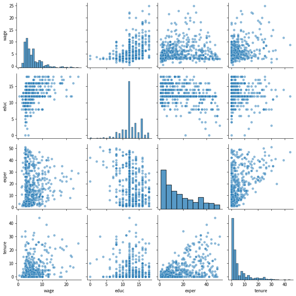
経験年数と対数賃金の相関係数は0.11であるが,経験年数と対数賃金の関係は線形というより,逆U字型である。すなわち,経験年数が増加すると賃金は上昇するが,その上昇率はだんだん小さくなっていき,一定の年齢を超えると賃金は低下する。また,経験年数が増加するほど修学年数が減少していることがわかる。これは,教育水準が上昇しており,経験年数の短い若い世代の労働者ほど修学年数が長いためである。
それでは最小二乗法による重回帰分析をやってみよう。
X = df[['educ', 'exper', 'female', 'nonwhite']]
y = df['wage']
X = sm.add_constant(X)  # 定数項を追加

model_multi = sm.OLS(y, X).fit()
print(model_multi.summary())
OLS Regression Results
==============================================================================
Dep. Variable: wage R-squared: 0.309
Model: OLS Adj. R-squared: 0.304
Method: Least Squares F-statistic: 58.34
Date: Thu, 15 Jan 2026 Prob (F-statistic): 1.09e-40
Time: 00:15:06 Log-Likelihood: -1335.7
No. Observations: 526 AIC: 2681.
Df Residuals: 521 BIC: 2703.
Df Model: 4
Covariance Type: nonrobust
==============================================================================
coef std err t P>|t| [0.025 0.975]
------------------------------------------------------------------------------
const -1.7145 0.762 -2.251 0.025 -3.211 -0.218
educ 0.6017 0.051 11.718 0.000 0.501 0.703
exper 0.0642 0.010 6.168 0.000 0.044 0.085
female -2.1565 0.271 -7.969 0.000 -2.688 -1.625
nonwhite -0.0839 0.444 -0.189 0.850 -0.957 0.789
==============================================================================
Omnibus: 198.454 Durbin-Watson: 1.813
Prob(Omnibus): 0.000 Jarque-Bera (JB): 782.640
Skew: 1.701 Prob(JB): 1.13e-170
Kurtosis: 7.913 Cond. No. 138.
==============================================================================
Notes:
[1] Standard Errors assume that the covariance matrix of the errors is correctly specified.推定結果を式で表すと, \[ \widehat{\log (wage)} = 0.53 + 0.098 educ + 0.010 exper \]
この式が意味するのは,
- 経験年数を一定として修学年数が1年増加すれば,時間あたり賃金が9.8%上昇する
- 修学年数を一定として経験年数が1年増加すれば,時間あたり賃金が1.0%上昇する
ということである。
単回帰の場合と重回帰の場合とで,修学年数の係数が異なることに注意しよう。これは,修学年数と経験年数が相関しているためである。若い労働者ほど修学年数が長いので,単回帰では修学年数が増加することの影響に,経験年数が短いことの影響が含まれてしまい,それによって修学年数の効果が小さく推定される。一方で,重回帰では,経験年数を一定とした修学年数の影響を計測しているため,係数が単回帰の場合に比べて大きくなっている。
経験年数と対数賃金の非線形 (逆U字型)の関係を捉えるため,経験年数の二乗項を加えた回帰式を考えよう。
\[ \widehat{\log (wage)} = \hat{\beta_0} + \hat{\beta_1} educ + \hat{\beta_2} exper + \hat{\beta_3}exper^2\]
この回帰式も最小二乗法によって推定することができる。そのためには,\(exper\)の二乗の変数を作成して,独立変数に加えれば良い。ここでは,データセットにもともと\(exper\)の二乗を計算した\(expersq\)が含まれているので,それを使う。
X = df[['educ', 'exper', 'expersq', 'female', 'nonwhite']]
y = df['lwage']
X = sm.add_constant(X)  # 定数項を追加

model_multi = sm.OLS(y, X).fit()
print(model_multi.summary())
OLS Regression Results
==============================================================================
Dep. Variable: lwage R-squared: 0.400
Model: OLS Adj. R-squared: 0.394
Method: Least Squares F-statistic: 69.26
Date: Thu, 15 Jan 2026 Prob (F-statistic): 1.89e-55
Time: 00:15:06 Log-Likelihood: -279.21
No. Observations: 526 AIC: 570.4
Df Residuals: 520 BIC: 596.0
Df Model: 5
Covariance Type: nonrobust
==============================================================================
coef std err t P>|t| [0.025 0.975]
------------------------------------------------------------------------------
const 0.3954 0.103 3.831 0.000 0.193 0.598
educ 0.0839 0.007 12.004 0.000 0.070 0.098
exper 0.0390 0.005 8.066 0.000 0.029 0.048
expersq -0.0007 0.000 -6.391 0.000 -0.001 -0.000
female -0.3374 0.036 -9.281 0.000 -0.409 -0.266
nonwhite -0.0213 0.060 -0.357 0.721 -0.139 0.096
==============================================================================
Omnibus: 7.115 Durbin-Watson: 1.774
Prob(Omnibus): 0.029 Jarque-Bera (JB): 10.541
Skew: 0.009 Prob(JB): 0.00514
Kurtosis: 3.693 Cond. No. 4.50e+03
==============================================================================
Notes:
[1] Standard Errors assume that the covariance matrix of the errors is correctly specified.
[2] The condition number is large, 4.5e+03. This might indicate that there are
strong multicollinearity or other numerical problems.推定結果から,\(exper\)の係数は0.041,\(exper^2\)の係数は-0.00071である。対数賃金と経験年数の関係は二次関数であり,経験年数がゼロのときには,経験年数が1年増加すれば4.1%賃金が上昇する。しかし,その上昇率は1年につき0.14%ずつ逓減していく。経験年数が約28年になると上昇率はマイナスとなり,賃金は経験年数とともに下がり始める。
対数賃金を独立変数を修学年数と経験年数,経験年数の二乗で説明しようとする回帰式をミンサー型賃金関数という。ミンサー型賃金関数は,どのような国のデータにも当てはまりが良く,一定の条件の下で修学年数の係数\(\hat{\beta_1}\)は,教育の内部収益率として解釈できる。