出生数と合計特殊出生率の推移

概要

人口動態調査を使って，1899年からの出生数の推移と，戦後の合計特殊出生率のグラフを描く。

コードと実行結果

library(tidyverse)
library(estatapi)
library(patchwork)

# e-statのappIDが必要
#   以下のページで利用申請(無料)をすればだれでも入手できる
#   https://www.e-stat.go.jp/api/
# appID = "入手したappIDをここに設定（行頭の#を外す）"

# グラフの軸を有効数字形式にする関数
# https://stats.biopapyrus.jp/r/ggplot/scientific-notation.html より

scientific_notation <- function(x) {
  x <- format(x, scientific = TRUE)
  x <- gsub("^(.*)e", "'\\1'e", x)
  x <- gsub("e", "%*%10^", x)
  x <- gsub("\\+", "", x)
  parse(text = x)
}

# e-Statからデータ取得
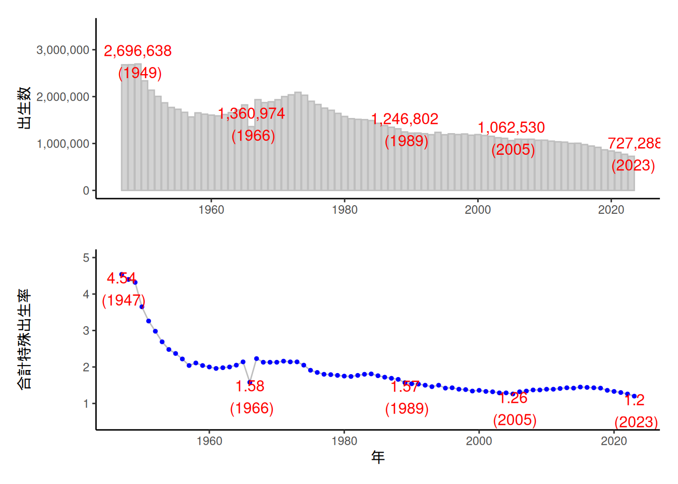
estat_vital <- estat_getStatsData(
  appId = appID,
  statsDataId = "0003411595", # 人口動態調査・人口動態統計・確定数・出生・4−1・上巻
  cdCat01 = c("00100", "00150")
)

Fetching record 1-244... (total: 244 records)

vital <- estat_vital |>
  mutate(
    year = as.numeric(time_code) / 1000000,
    name = `出生数・出生率・出生性比`
  ) |>
  select(year, name, value) |>
  filter(year >= 1947) |>
  pivot_wider(names_from = name)

# グラフ作成
birth <- vital |>
  ggplot(
    aes(
      x = year,
      y = `出生数_総数`
    )
  ) +
  geom_bar(
    stat = "identity",
    color = "gray",
    fill = "lightgray"
  ) +
  scale_y_continuous(
    labels = scientific_notation,
    limits = c(0, 3500000)
  ) +
  geom_text(
    aes(
      label = paste(
        format(`出生数_総数`, big.mark = ","),
        "\n (", year, ")",
        sep = ""
      )
    ),
    nudge_y = 50000,
    color = "red",
    size = 4,
    data = subset(vital, year %in% c(1949, 1966, 1989, 2005, 2023))
  ) +
  labs(
    x = "",
    y = "出生数"
  )

tfr <- vital |>
  ggplot(
    aes(
      x = year,
      y = `合計特殊出生率`
    )
  ) +
  geom_line(color = "gray") +
  geom_point(
    size = 1,
    color = "blue"
  ) +
  ylim(0.5, 5) +
  geom_text(
    aes(
      label = paste(`合計特殊出生率`, "\n (", year, ")",
      sep = "")),
    nudge_y = -0.4,
    color = "red",
    size = 4,
    data = subset(vital, year %in% c(1947, 1966, 1989, 2005, 2023))
  ) +
  labs(
    x = "年",
    y = "合計特殊出生率"
  )

# patchworkパッケージを使ったプロット
birth + tfr + plot_layout(ncol = 1)