労働力率の推移

概要

労働力調査を用いて，労働力人口の推移，年齢階級別労働力率・失業率の推移，労働供給のM字カーブのグラフを作成する。

コードと実行結果

library(tidyverse)
library(estatapi)
library(readxl)
library(RColorBrewer)
library(patchwork)

# e-statのappIDが必要
#   以下のページで利用申請(無料)をすればだれでも入手できる
#   https://www.e-stat.go.jp/api/
# appID = "入手したappIDをここに設定（行頭の#を外す）"

# グラフのテーマ
theme_set(theme_classic(base_family = "IPAexGothic", base_size = 16))

# ファイルのダウンロード先ディレクトリ作成
dir.create("files", showWarnings = FALSE)

# e-statからファイルのダウンロード

# 人口推計 長期時系列データ 我が国の推計人口（大正9年～平成12年）
download.file(
  "https://www.e-stat.go.jp/stat-search/file-download?statInfId=000000090261&fileKind=0",
  destfile = "files/pop_estimate1920-2000.xlsx",
  method = "curl"
)

# 人口推計 長期時系列データ（平成12年～令和２年）
download.file(
  "https://www.e-stat.go.jp/stat-search/file-download?statInfId=000013168601&fileKind=4",
  destfile = "files/pop_estimate2000-2020.xlsx",
  method = "curl"
)

# 総人口データの結合

pop_1 <- read_excel(
  "files/pop_estimate1920-2000.xlsx",
  range = "D11:D90",
  col_names = FALSE
)

pop_2 <- read_excel(
  "files/pop_estimate2000-2020.xlsx",
  sheet = 1, 
  range = "D11:D25", 
  col_names = FALSE
)

pop_3 <- read_excel(
  "files/pop_estimate2000-2020.xlsx", 
  sheet = 2, 
  range = "C11:C15", 
  col_names = FALSE
)

pop_4 <- estat_getStatsData(
  appId = appID,
  statsDataId = "0003448228", # 人口推計 各年10月1日現在人口 令和２年国勢調査基準 統計表 表番号001
  cdCat01 = "001", # 男女計
  cdCat02 = "001", # 総人口
  cdCat03 = "01000" # 総数
) |>
  rename(...1 = value) |>
  select(...1)

population <- cbind(
  seq(1920, 2019 + nrow(pop_4), 1),
  rbind(pop_1, pop_2, pop_3, pop_4) / 10,
  "総人口"
)

colnames(population) <- c("year", "value", "category")

# 労働力調査　基本集計　全都道府県　年次　表番号1-1-5

labor_force <- estat_getStatsData(
  appId = appID,
  statsDataId = "0002060047",
  cdCat01 = "000", # 全産業
  cdCat03 = c("00", "01", "08"), # 15歳以上人口，労働力人口，完全失業者
  cdArea = "00000" # 全国
) |>
  mutate(year = as.numeric(time_code) / 1000000) |>
  select(year, `性別`, `就業状態`, `年齢階級`, `value`)

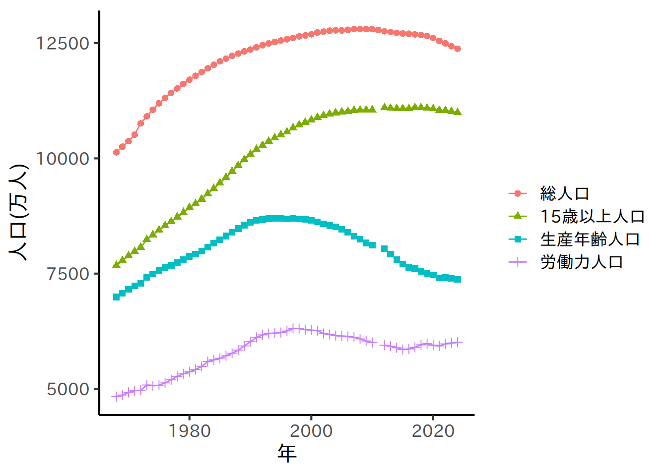
# 総人口と労働力人口の推移

population_laborforce <- rbind(
  labor_force |>
    mutate(
      category = factor(
        case_when(
          `就業状態` == "15歳以上人口" & `年齢階級` == "15歳以上" ~ "15歳以上人口",
          `就業状態` == "15歳以上人口" & `年齢階級` == "15～64歳" ~ "生産年齢人口",
          `就業状態` == "労働力人口" & `年齢階級` == "15～64歳" ~ "労働力人口",
          TRUE ~ ""
        ),
        levels = c(
          "総人口", "15歳以上人口",
          "生産年齢人口", "労働力人口"
        )
      )
    ) |>
    filter(`性別` == "総数" & category != "") |>
    select(year, value, category),
  population
)

# グラフ作成
graph_population_laborforce <- population_laborforce |>
  filter(year >= 1968) |>
  ggplot(
    aes(
      x = year, 
      y = value, 
      color = category, 
      shape = category
    )
  ) +
  geom_line() +
  geom_point(size = 2) +
  scale_color_discrete(name = "") +
  scale_shape_discrete(name = "") +
  labs(x = "年", y = "人口(万人)")

plot(graph_population_laborforce)

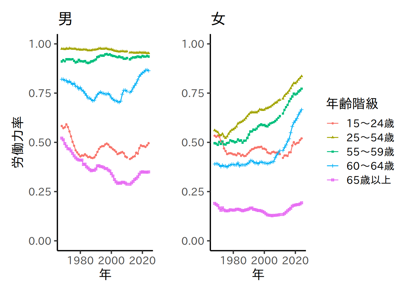
# 年齢階級別労働力率

# データ整理
lf_by_age <- labor_force |>
  filter(year >= 1968) |>
  pivot_wider(names_from = `年齢階級`) |>
  mutate(`25～54歳` = `25～34歳` + `35～44歳` + `45～54歳`) |> # 25~54歳までをまとめる
  pivot_longer(
    - c("year", "性別", "就業状態"),
    names_to = "年齢階級"
  ) |>
  pivot_wider(
    names_from = `就業状態`
  ) |>
  mutate(
    participation_rate = `労働力人口` / `15歳以上人口`,
    unemployment_rate = `完全失業者` / `労働力人口`
  )

# グラフ作成
age_groups <- c("15～24歳", "25～54歳", "55～59歳", "60～64歳", "65歳以上")

graph_male_age <- lf_by_age |>
  filter(`性別` == "男" & `年齢階級` %in% age_groups) |>
  ggplot(
    aes(
      x = year,
      y = participation_rate,
      color = `年齢階級`,
      shape = `年齢階級`
    )
  ) +
  geom_line() +
  geom_point(size = 1) +
  ylim(0, 1) +
  labs(
    title = "男",
    x = "年",
    y = "労働力率"
  ) +
  theme(legend.position = "none")

graph_female_age <- lf_by_age |>
  filter(`性別` == "女" & `年齢階級` %in% age_groups) |>
  ggplot(
    aes(
      x = year, 
      y = participation_rate,
      color = `年齢階級`, 
      shape = `年齢階級`
    )
  ) +
  geom_line() +
  geom_point(size = 1) +
  ylim(0, 1) +
  labs(
    title = "女",
    x = "年",
    y = ""
  )

plot(graph_male_age + graph_female_age)

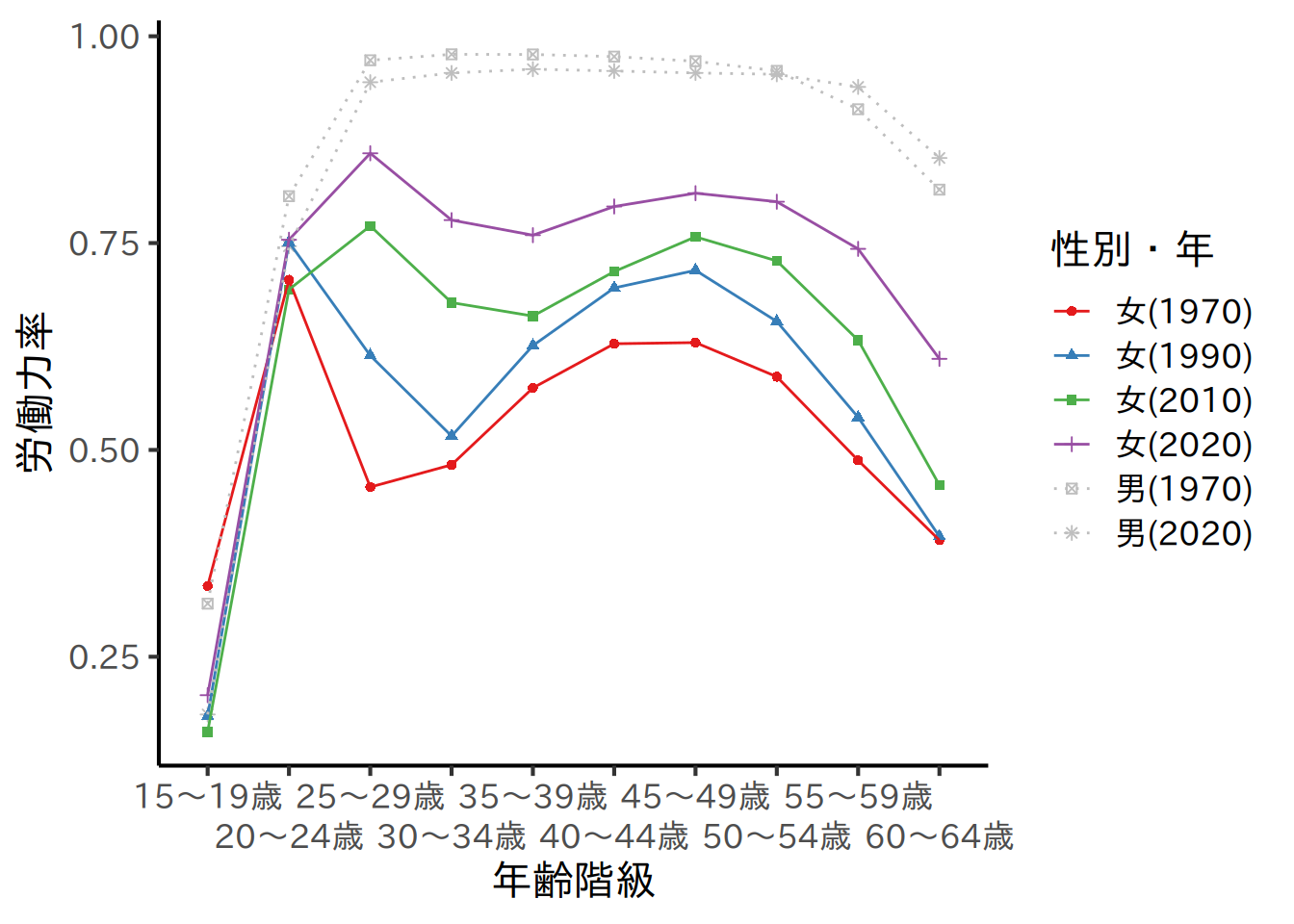
# M字カーブ

# データ整理
years <- c(1970, 1990, 2010, 2020)

age_groups <- c(
  "15～19歳", 
  "20～24歳", 
  "25～29歳", 
  "30～34歳", 
  "35～39歳",
  "40～44歳", 
  "45～49歳", 
  "50～54歳", 
  "55～59歳", 
  "60～64歳"
)

m_curve <- lf_by_age |>
  filter(
    (`性別` == "女" & year %in% years & `年齢階級` %in% age_groups) | # 女性
    (`性別` == "男" & year %in% c(years[1], years[length(years)]) &
    `年齢階級` %in% age_groups) # 男性は最初と最後の年のみ
  ) |>
  mutate(`性別・年` = paste(`性別`, "(", year, ")", sep = ""))

# グラフ作成
graph_m_curve <- m_curve |>
  ggplot(
    aes(
      x = `年齢階級`,
      y = participation_rate,
      color = `性別・年`,
      linetype = `性別・年`,
      shape = `性別・年`, 
      group = `性別・年`
    )
  ) +
  geom_point() +
  geom_line() +
  scale_color_manual(
    values = c(brewer.pal(4, "Set1"), "grey", "grey")
  ) +
  scale_x_discrete(
    guide = guide_axis(n.dodge = 2)
  ) +
  scale_linetype_manual(
    values = c(
      "solid",
      "solid",
      "solid",
      "solid",
      "dotted",
      "dotted"
    )
  ) +
  labs(y = "労働力率")

plot(graph_m_curve)