職業構成の変化 (労働力調査)

概要

労働力調査の長期時系列データから，就業者の職業構成の変化をグラフ化する。

2009年の日本標準職業分類の変更に伴い，データはその前後で完全には接続できない。ここでは，新旧の分類を統合せず，それぞれについてグラフを作成する。

なお，職業構成の変化は国勢調査からも確認できる。

コードと実行結果

library(tidyverse)
library(ggrepel)
library(readxl)

theme_set(theme_classic(base_family = "IPAexGothic", base_size = 12))

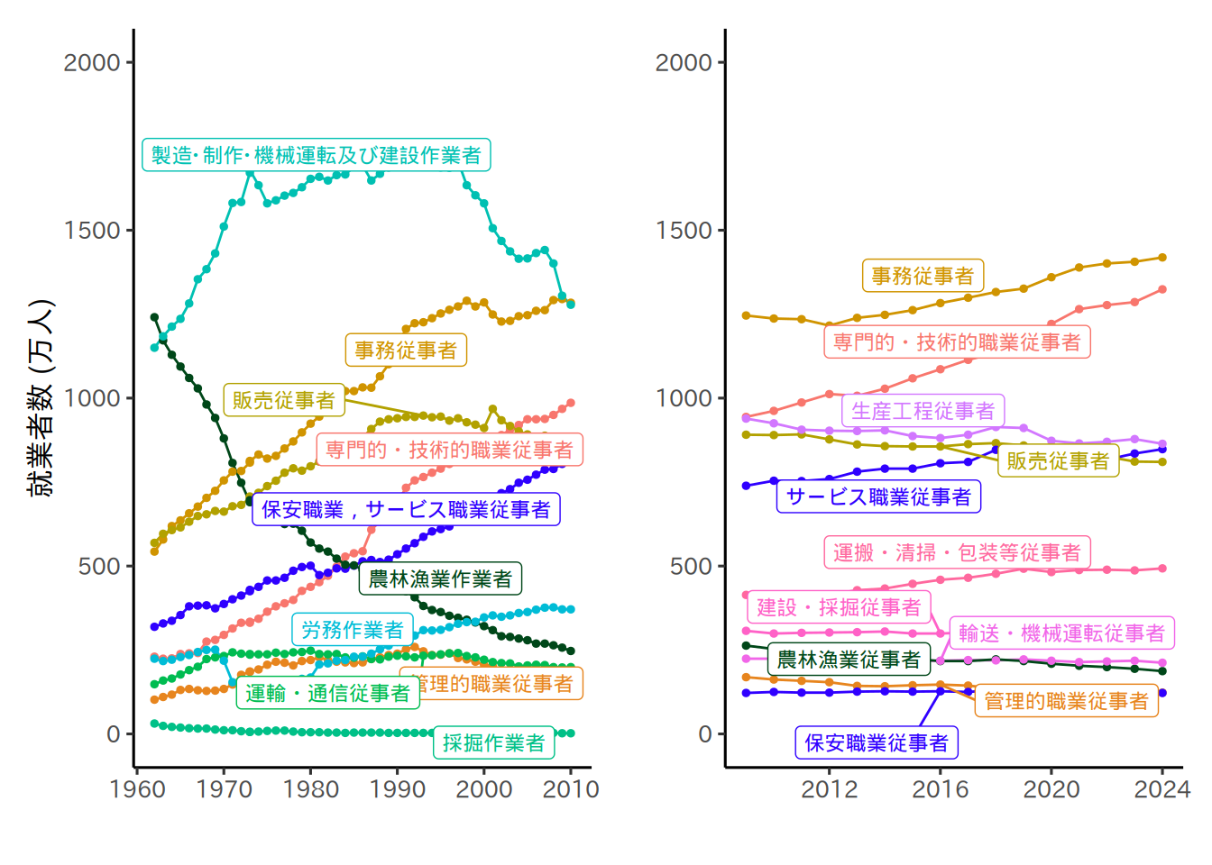
# 労働力調査　長期時系列【表６】年平均結果 6-2 職業別就業者数
download.file(
  "https://www.e-stat.go.jp/stat-search/file-download?statInfId=000001082694&fileKind=0",
  destfile = "files/occupation_6-2.xls",
  method = "curl"
)

header <- read_excel(
  "files/occupation_6-2.xls",
  range = "C6:M6",
  col_names = FALSE
)
header <- c("year", gsub("\\s+", "", unname(unlist(header))))

data <- read_excel(
  "files/occupation_6-2.xls",
  range = "B18:M67",
  col_names = FALSE
)

colnames(data) <- header

long_data_1 <- data %>%
  select(- `総数`) |>
  pivot_longer(cols = c(- year), names_to = "occupation")


# 労働力調査　長期時系列【表６】年平均結果 6-1 職業別就業者数（2009年12月改定分類）
download.file(
  "https://www.e-stat.go.jp/stat-search/file-download?statInfId=000012925012&fileKind=0",
  destfile = "files/occupation_6-1.xlsx",
  method = "curl"
)

header <- read_excel(
  "files/occupation_6-1.xlsx",
  range = "C6:N6",
  col_names = FALSE
)
header <- c("year", gsub("\\s+", "", unname(unlist(header))))


data <- read_excel(
  "files/occupation_6-1.xlsx",
  range = "B9:N24",
  col_names = FALSE
)

colnames(data) <- header

long_data_2 <- data %>%
  select(- `総数`) |>
  pivot_longer(cols = c(- year), names_to = "occupation")


# 色を指定
fixed_cols <- c(
  "保安職業従事者"   = "#2f00ff",
  "サービス職業従事者" = "#2f00ff",
  "保安職業，サービス職業従事者" = "#2f00ff",
  "農林漁業従事者" = "#004719",
  "農林漁業作業者" = "#004719"
)

# 全職業の一覧を作成し、ベースの色を用意
all_occ <- union(unique(long_data_1$occupation), unique(long_data_2$occupation))
base_pal <- setNames(scales::hue_pal()(length(all_occ)), all_occ)


# 固定色で上書き（存在すれば置換）
for (k in names(fixed_cols)) {
  if (k %in% names(base_pal)) base_pal[k] <- fixed_cols[k]
}

g1 <- long_data_1 %>%
  ggplot(aes(x = year, y = value, color = occupation, group = occupation)) +
  geom_line() +
  geom_point(size = 1) +
  ylim(0, 2000) +
  labs(x = "", y = "就業者数 (万人)") +
  geom_label_repel(
    data = filter(long_data_1, year == 1993),
    aes(label = occupation),
    size = 3, show.legend = FALSE
  ) +
  scale_color_manual(values = base_pal, limits = all_occ, drop = FALSE) +
  theme(legend.position = "none")

g2 <- long_data_2 %>%
  ggplot(aes(x = year, y = value, color = occupation, group = occupation)) +
  geom_line() +
  geom_point(size = 1) +
  ylim(0, 2000) +
  labs(x = "", y = "") +
  geom_label_repel(
    data = filter(long_data_2, year == 2016),
    aes(label = occupation),
    size = 3, show.legend = FALSE
  ) +
  scale_color_manual(values = base_pal, limits = all_occ, drop = FALSE) +
  theme(legend.position = "none")

plot(g1 + g2)